opencv边缘检测 C++实现
1 opencv C++ 环境配置
1.1 C++环境安装
visual studio 2019 community version 下载地址: https://visualstudio.microsoft.com/zh-hans/vs/community/
双击安装包进入安装界面,选择C++开发包之后点击安装,等待程序安装完成。
原图床图片已失效(
visual) 原链接https://s2.ax1x.com/2020/02/12/1Hjlh6.png已被图床删除。
1.2 opencv环境配置
1.2.1 opencv 下载
安装包 下载地址:https://sourceforge.net/projects/opencvlibrary/files/4.2.0/opencv-4.2.0-vc14_vc15.exe/download
双击安装包进入安装界面,并将其安装到一个方便你找到的文件夹中。比如:C:\opencv,之后的opencv目录将以该目录作为安装根目录为例。
1.2.2 环境变量配置
1 打开控制面板 - 所有控制面板项 - 系统。
2 点击左侧的高级系统设置。
3 选择右下的环境变量。
4 双击下方系统变量的Path。
5 在Path中新建一个环境变量,地址是C:\opencv\build\x64\vc15\bin。
6 连点应用确认完成配置
原图床图片已失效(
环境变量) 原链接https://s2.ax1x.com/2020/02/12/1HjE1U.png已被图床删除。
1.2.3 VS2019环境配置
1 打开VS2019,create new project - 选择C++ - 选择empty project。
原图床图片已失效(
emptyproject) 原链接https://s2.ax1x.com/2020/02/12/1Hjr38.png已被图床删除。
2 进入主界面之后,点击左上角view - other windows - property manager,调出属性管理器。
原图床图片已失效(
propertymanager) 原链接https://s2.ax1x.com/2020/02/12/1Hj2Hs.png已被图床删除。
3 在属性管理器的Debug | 64选项右键选择Properties。
原图床图片已失效(
debug) 原链接https://s2.ax1x.com/2020/02/12/1HvnxS.png已被图床删除。
4 在Debug Property Pages界面左侧选择VC++ Directories,将右侧的Include Directories添加C:\opencv\build\include, 将Library Directories添加C:\opencv\build\x64\vc15\lib。
原图床图片已失效(
includelib) 原链接https://s2.ax1x.com/2020/02/12/1Hv3an.png已被图床删除。
5 在Debug Property Pages界面左侧选择Linker,将右侧的Additional Dependencies添加opencv_world420.lib。
原图床图片已失效(
linker) 原链接https://s2.ax1x.com/2020/02/12/1Hvt2T.png已被图床删除。
*若你装的版本不是4.2.0,则将420换为你安装的版本的版本号。
6 之后关闭Debug Property Pages界面,确认VS主界面上方的Debug使用的是x64版本,若不是则选择x64。
原图床图片已失效(
x64) 原链接https://s2.ax1x.com/2020/02/12/1HvTit.png已被图床删除。
至此,整个C++ opencv 的VS环境配置完毕。 顺便,该配置只针对当前创建的Project有效,若创建新的Project后,需重新进行以上配置。
2 opencv的基本输入输出以及指针调用
2.1 头文件
#include <opencv2/opencv.hpp>   //opencv头文件
#include <iostream> //C++基本输入输出

//名空间声明
using namespace cv;
using namespace std;
2.2 图像IO
2.2.1 图像输入
Mat In = imread("C:\\test.png", IMREAD_GRAYSCALE);imread函数是opencv库中的基本输入函数,可以将.png.jpg.bmp等格式的图片读入,并转化为opencv的图片矩阵类型Mat。 imread的第一个输入变量为文件的具体位置,第二个变量IMREAD_GRAYSCALE表示读入灰度图,若不加这条则会读入RGB图。
2.2.2 图像复制
在opencv中,如果使用赋值手法进行图像的复制,如下所示:
Mat Out = In;则会将In的每个像素位置的指针赋给Out,不论对In还是Out进行修改时,另外一个变量也会跟着进行变化。 因此,想要进行图像复制要用Mat类型的clone()方法:
Mat Out = In.clone;2.2.3 图像显示输出
imshow("Output", Out);imshow函数是opencv库中的基本输出函数,可以将Mat类型的图像显示在屏幕上。 imshow的第一个变量是图像显示在屏幕上的文本内容,第二个变量是选择输出的Mat类型变量。
原图床图片已失效(
imshow示例截图) 原链接https://s2.ax1x.com/2020/02/12/1HxGeH.png已被图床删除。
*注意:如果两个输出图像的文本相同则只会输出先输出的一个图像,因此不要将输出图像的文本定义为一样的文本。
2.2.4 图像保存输出
imwrite("C:\\Out.png", Output);imwrite函数是opencv库的基本输出函数,可以进行指定目录的图片写入功能。 imwrite的第一个变量是保存输出图片的具体位置,第二个变量是选择输出的Mat类型的变量。
2.3 图片的特定像素提取
下面以一个阈值法进行边缘检测为例说明像素提取的方法:
    Mat Output = Input.clone();
    for (int x = 1; x < Input.rows - 1; x++)
    {
        uchar* out = Output.ptr<uchar>(x);
        uchar* current = Input.ptr<uchar>(x);
        uchar* last = Input.ptr<uchar>(x - 1);
        for (int y = 1; y < Input.cols - 1; y++)
        {
            if (abs(current[y] - current[y - 1]) > K || abs(current[y] - last[y]) > K)  //Threshold K
            {
                out[y] = 255;
                continue;
            }
            else
            {
                out[y] = 0;
            }
        }
    }
其中,
uchar* out = Output.ptr<uchar>(x);表示将第 x 行的第一个像素指针赋给out。
out[y] = 255;表示将第 x 行的第 y 个像素值赋值255。
另外,上述像素操作建立在灰度图的基础上。若对于RGB彩色图,官方的Mat类型将以下图形式存储像素值数据 [1]:
原图床图片已失效(
out) 原链接https://s2.ax1x.com/2020/02/12/1HxfpV.png已被图床删除。
[1]https://docs.opencv.org/master/db/da5/tutorial_how_to_scan_images.html
3 边缘检测算法
3.1 阈值法
流程图:
原图床图片已失效(
Threshold_flow) 原链接https://s2.ax1x.com/2020/02/12/1HzOEj.jpg已被图床删除。
代码:
void Threshold_Method(Mat Input, int K)
{
    Mat Output = Input.clone();
    for (int x = 1; x < Input.rows - 1; x++)
    {
        uchar* sum = Output.ptr<uchar>(x);
        uchar* current = Input.ptr<uchar>(x);
        uchar* last = Input.ptr<uchar>(x - 1);
        for (int y = 1; y < Input.cols - 1; y++)
        {
            if (abs(current[y] - current[y - 1]) > K || abs(current[y] - last[y]) > K)  //Threshold K
            {
                //sum[y] = 255;
                continue;
            }
            else
            {
                sum[y] = 0;
            }
        }
    }
    imshow("Threshold_Method", Output);
}
结果:
原图床对比图已失效(原图与阈值法结果)原链接
https://s2.ax1x.com/2020/02/12/1bSyin.png、https://s2.ax1x.com/2020/02/12/1bSAa9.png已被图床删除。
3.2 差分法
流程图:
原图床图片已失效(
Difference_flow) 原链接https://s2.ax1x.com/2020/02/12/1bSOsO.jpg已被图床删除。
代码:
void Difference_Method(Mat Input)
{
    Mat Output = Input.clone();
    for (int x = 1; x < Input.rows - 1; x++)
    {
        uchar* sum = Output.ptr<uchar>(x);
        uchar* current = Input.ptr<uchar>(x);
        uchar* last = Input.ptr<uchar>(x - 1);
        for (int y = 1; y < Input.cols - 1; y++)
        {
            float horizontal = pow(current[y] - current[y - 1], 2);
            float vertical = pow(current[y] - last[y], 2);
            sum[y] = saturate_cast<uchar>(sqrt(horizontal + vertical));   //output = sqrt(delta_x ^ 2 + delta_y ^ 2)
        }
    }
    imshow("Difference_Method", Output);
}
结果:
原图床对比图已失效(原图与差分法结果)原链接
https://s2.ax1x.com/2020/02/12/1bSyin.png、https://s2.ax1x.com/2020/02/12/1bpky8.png已被图床删除。
3.3 Sobel方法
流程图:
原图床图片已失效(
Sobel) 原链接https://s2.ax1x.com/2020/02/12/1bpQS0.jpg已被图床删除。
代码:
void Sobel_Method(Mat Input, const char* Str)
{
    Mat Output = Input.clone();
    for (int x = 1; x < Input.rows - 1; x++)
    {
        uchar* sum = Output.ptr<uchar>(x);
        uchar* current = Input.ptr<uchar>(x);
        uchar* next = Input.ptr<uchar>(x + 1);
        uchar* last = Input.ptr<uchar>(x - 1);
        for (int y = 1; y < Input.cols - 1; y++)
        {
            /*
            horizontal
            [ -1  0  1
              -2  0  2
              -1  0  1 ]
            */
            float horizontal = pow(-last[y - 1] + last[y + 1]
                - 2 * current[y - 1] + 2 * current[y + 1]
                - next[y - 1] + next[y + 1]
                , 2);

            /*
            vertical
            [ -1 -2 -1
               0  0  0
               1  2  1 ]
            */
            float vertical = pow(-last[y - 1] - 2 * last[y] - last[y + 1]
                + next[y - 1] + 2 * next[y] + next[y + 1]
                , 2);
            sum[y] = saturate_cast<uchar>(sqrt(horizontal + vertical));

        }
    }
    imshow(Str, Output);
}
结果:
原图床对比图已失效(原图与 Sobel 结果)原链接
https://s2.ax1x.com/2020/02/12/1bSyin.png、https://s2.ax1x.com/2020/02/12/1bpB6K.png已被图床删除。
3.4 拉普拉斯方法
流程图:
原图床图片已失效(
Laplacian_flow) 原链接https://s2.ax1x.com/2020/02/12/1bph1P.jpg已被图床删除。
代码:
void Laplacian_Method(Mat Input, const char* Str)
{
    Mat Output = Input.clone();
    for (int x = 1; x < Input.rows - 1; x++)
    {
        uchar* sum = Output.ptr<uchar>(x);
        uchar* current = Input.ptr<uchar>(x);
        uchar* next = Input.ptr<uchar>(x + 1);
        uchar* last = Input.ptr<uchar>(x - 1);
        for (int y = 1; y < Input.cols - 1; y++)
        {
            /*
            [ 0  1  0
              1 -4  1
              0  1  1 ]
            */
            sum[y] = saturate_cast<uchar>(last[y]
                + current[y - 1] - 4 * current[y] + current[y + 1]
                + next[y]) * 20;

        }
    }
    imshow(Str, Output);
}
结果:
原图床对比图已失效(原图与拉普拉斯结果)原链接
https://s2.ax1x.com/2020/02/12/1bSyin.png、https://s2.ax1x.com/2020/02/12/1bpLhn.png已被图床删除。
3.5 高斯滤波
流程图:
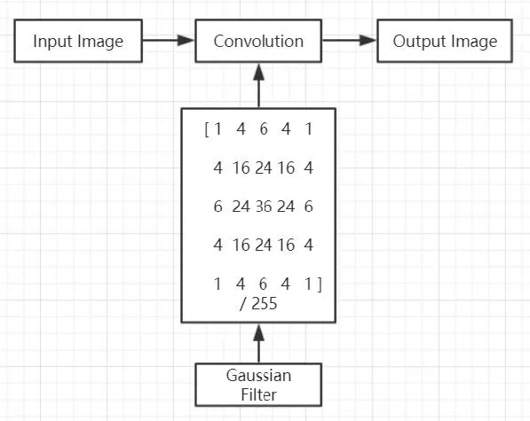
代码:
Mat Gaussian_Filter_5(Mat Input, int K)
{
    Mat Output = Input.clone();
    for (int k = 1; k < K + 1; k++)
    {
        Mat Output_buff = Output.clone();
        for (int x = 2; x < Input.rows - 2; x++)
        {
            uchar* sum = Output.ptr<uchar>(x);
            uchar* current = Output_buff.ptr<uchar>(x);
            uchar* next = Output_buff.ptr<uchar>(x + 1);
            uchar* next_ = Output_buff.ptr<uchar>(x + 2);
            uchar* last = Output_buff.ptr<uchar>(x - 1);
            uchar* last_ = Output_buff.ptr<uchar>(x - 2);
            for (int y = 2; y < Input.cols - 2; y++)
            {
                /*
                [ 1  4  6  4  1
                  4 16 24 16  4
                  6 24 36 24  6
                  4 16 24 16  4
                  1  4  6  4  1 ]
                */
                sum[y] = saturate_cast<uchar>((+1 * last_[y - 2] + 4 * last_[y - 1] + 6 * last_[y] + 4 * last_[y + 1] + 1 * last_[y + 2]
                    + 4 * last[y - 2] + 16 * last[y - 1] + 24 * last[y] + 16 * last[y + 1] + 4 * last[y + 2]
                    + 6 * current[y - 2] + 24 * current[y - 1] + 36 * current[y] + 24 * current[y + 1] + 6 * current[y + 2]
                    + 4 * next[y - 2] + 16 * next[y - 1] + 24 * next[y] + 16 * next[y + 1] + 4 * next[y + 2]
                    + 1 * next_[y - 2] + 4 * next_[y - 1] + 6 * next_[y] + 4 * next_[y + 1] + 1 * next_[y + 2]) * 0.00390625);

            }
        }
    }
    return Output;
}
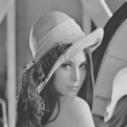
结果:
原对比左图(原图
https://s2.ax1x.com/2020/02/12/1bSyin.png)已被图床删除,以下为处理结果图:
3.6 高斯滤波后的Sobel
流程图:

代码:
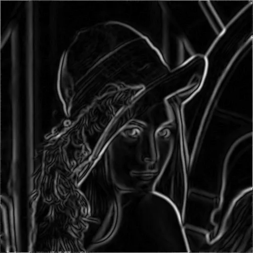
Sobel_Method(Gaussian_Filter_5(In, 2), "Sobel_Method_with_Gaussian_Filter");结果:
原对比左图(原图
https://s2.ax1x.com/2020/02/12/1bSyin.png)已被图床删除,以下为处理结果图:
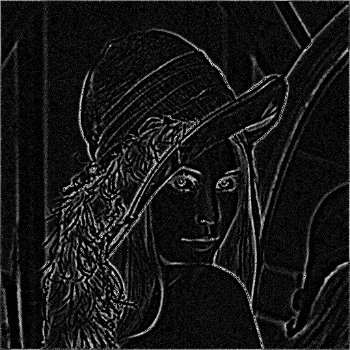
3.7 高斯滤波后的拉普拉斯方法
流程图:

代码:
Laplacian_Method(Gaussian_Filter_5(In, 2), "Laplacian_Method_with_Gaussian_Filter");结果:
原对比左图(原图
https://s2.ax1x.com/2020/02/12/1bSyin.png)已被图床删除,以下为处理结果图:
3.8 基于拉普拉斯方法的锐化算法
流程图:
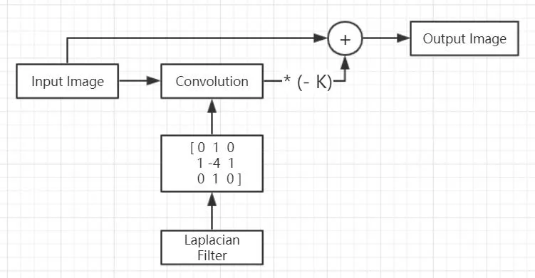
代码:
void Sharpening_based_on_Laplacian(Mat Input, int K)
{
    Mat Output = Input.clone();
    for (int x = 1; x < Input.rows - 1; x++)
    {
        uchar* sum = Output.ptr<uchar>(x);
        uchar* current = Input.ptr<uchar>(x);
        uchar* next = Input.ptr<uchar>(x + 1);
        uchar* last = Input.ptr<uchar>(x - 1);
        for (int y = 1; y < Input.cols - 1; y++)
        {
            /*
            [   0         - K    0
              - K  (1 + 4 * K)  - K
                0         - K    0 ]
            */
            sum[y] = saturate_cast<uchar>(
                -K * last[y]
                - K * current[y - 1] + (1 + 4 * K) * current[y] - K * current[y + 1]
                - K * next[y]);
        }
    }
    imshow("Sharpening_based_on_Laplacian", Output);
}
结果:
原对比左图(原图
https://s2.ax1x.com/2020/02/12/1bSyin.png)已被图床删除,以下为处理结果图: